
Spring Transition Dates and Fall Transition Dates
OSCURS Method
Method & Data Reference
Ingraham, W.J., Jr. and R. K. Miyihara. 1988. Ocean surface current simulations in the North Pacific Ocean and Bering Sea (OSCURS-Numerical Model). NOAA Tech. Mem., NMFS F/ NWC-130, 155 p.
Summary
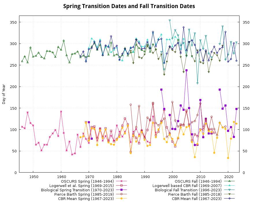
Each year, along the Pacific Coast of North American between San Francisco (38 North Latitude) and the Queen Charlotte Islands (52 North
Latitude), the coastal winds switch from the southerly winds of winter
to the northerly winds of summer producing a transition in wind called
the spring transition. Conversely, the yearly switch back from the
northerly winds of summer to the southerly winds of winter produce a
fall transition. The summer winds, which occur after the spring
transition and prior to the fall transition, are known to be favorable
for upwelling
Disclaimer
The dates of the spring and fall transitions contained on the web page should be considered provisional. They are values which are approximations to the true spring and fall transition dates. The estimates depend on the degree and type of smoothing used on the synthetic winds derived from OSCURS. Neither NOAA nor the University of Washington is responsible for any misuse of these data.
Logerwell et al. Method
Method Reference
Logerwell, E.A., N. Mantua, P. Lawson, R.C. Francis, V. Agostini. 2003. Tracking environmental processes in the coastal zone for understanding and predicting Oregon coho (Oncorhynchus kisutch) marine survival. Fisheries Oceanography 12:554-568.
Data Reference
E. Logerwell (pers. com. 2007)
Summary
The date of spring transition can be indexed in several ways; the Logerwell et al. (2003) method indexes the spring transition date based on the first day when the value of the 10-day running average for upwelling is positive and the 10-day running average for sea level is negative.
Disclaimer
Transitions dates contained on the web page should be considered provisional. They are values which are approximations to the true spring and fall transition dates. Neither NOAA nor the University of Washington is responsible for any misuse of these data.
Biological Spring and Fall Transition Method
Primary Source and Summary
Please refer to Local Biological Indicators, NOAA Fisheries for the official documentation and dataset. Data last accessed: 12 January 2026.
Contacts
Cheryl Morgan
Cooperative Institute for Marine Ecosystem and Resources
Oregon State University
Hatfield Marine Research Station
2032 S Marine Science Drive
Newport, Oregon 97365-5275
cheryl.morgan@noaa.gov
Samantha Zeman
Cooperative Institute for Marine Ecosystem and Resources
Oregon State University
Hatfield Marine Research Station
2032 S Marine Science Drive
Newport, Oregon 97365-5275
zemans@oregonstate.edu
Pierce and Barth Method
Method Reference
Barth, J. A., B. A. Menge, J. Lubchenco, F. Chan, J. M. Bane, A. R. Kirincich, M. A. McManus, K. J. Nielsen, S. D. Pierce, and L. Washburn (2007) Delayed upwelling alters nearshore coastal ocean ecosystems in the northern California current, Proceedings of the National Academy of Sciences, 104, 3719-3724.
Gustafsson, F. (2000) Adaptive filtering and change detection, John Wiley.
Hinkley, D. and E. Schechtman (1987) Conditional bootstrap methods in the mean-shift model. Biometrika, 74, 85-93.
Huyer, A., E. J. C. Sobey, and R. L. Smith (1979) The spring transition in currents over the Oregon continental shelf. J. Geophys. Res., 84, 6995-7011.
Large, W. G. and S. Pond (1981) Open ocean momentum flux measurements in moderate-to-strong winds. J. Phys. Oc., 11, 324-336.
Page, E. S. (1954) Continuous inspection schemes. Biometrika, 41, 100-115.
Pierce, S. D., J. A. Barth, R. E. Thomas, and G. W. Fleischer (2006) Anomalously warm July 2005 in the northern California Current: historical context and the significance of cumulative wind stress, Geophys. Res. Letters, 33, L22S04, doi:10.1029/2006GL027149.
Summary from "Wind stress, cumulative wind stress, and spring transition dates: data products for Oregon upwelling-related research "
Alongshore wind stress cumulative from the spring transition represents energy input into the upwelling system over the course of each season. This has been found to be strongly correlated with a number of different upwelling metrics (Pierce et al., 2006), eg. NH-line surface-layer temperature (0-30m).
Wind stress here is derived from observed winds at Newport, Oregon, using the method of Large and Pond (1981). The hourly data are low-pass filtered to remove diurnal variations. The spring and fall transitions (Huyer et al., 1979) are estimated for each year from the alongshore wind stress record, using a CUSUM algorithm for change-point detection (Page, 1954; Gustafsson, 2000). The significance (95%) of these two mean-shift change-points within each year's time series is confirmed using bootstrapping, as suggested by Hinkley and Schechtman (1987).
We hope that researchers will find it useful to compare their own upwelling-related data to the general development of upwelling represented by this cumulative wind stress product. Plots and data are available: Wind stress, cumulative wind stress, and spring transition dates: data products for Oregon upwelling-related research.
S. D. Pierce and J. A. Barth, College of Earth, Ocean, & Atmospheric Sciences
Logerwell based CBR Method
Method Reference
Logerwell, E.A., N. Mantua, P. Lawson, R.C. Francis, V. Agostini. 2003. Tracking environmental processes in the coastal zone for understanding and predicting Oregon coho (Oncorhynchus kisutch) marine survival. Fisheries Oceanography 12:554-568.
Bilbao, P. 1999. Interannual and Interdecadal Variability in the Timing and Strength of the Spring Transitions along the United States West Coast. M.S. Thesis. Oregon State University, Oceanography.
Summary
The method is the same as that used in Logerwell (2003) to estimate spring transition dates.
Two time series were inspected for seasonal transitions: (1) area averaged daily upwelling indices for 42º to 48ºN, 125ºW (Environmental Research Data Services, NOAA Fisheries), and (2) daily sea level residuals (corrected for the inverse barometer effect) measured at Neah Bay, WA, 48º22.1'N,124º37.0'W ( University of Hawaii Sea Level Center). High frequency variation was filtered out by applying a low pass filter with a stop frequency of 1/(10 days) (S-PLUS, MathSoft, Inc., Seattle, WA, USA). To extract the seasonal pattern, a low pass filter with a stop frequency of 1/(90 days) was constructed. The date of fall transition was chosen as the date when the 1/(10 days) low pass filtered lines crossed zero.� The 1/(90 days) low pass filter line confirmed that the selected date marked the beginning of a new seasonal state.
In most years the time series agree and the date is easy to pick. In other years the signals do not point to a single transition and some judgment must be made. Thus, although the model allows selection of the date, it does not form a completely objective and automated system for choosing that date.
Update
13 April 2007. Estimates for 1997, 2000, and 2004 were updated.
Disclaimer
Transitions dates contained on the web page should be considered provisional. They are values which are approximations to the true spring and fall transition dates. The University of Washington is not responsible for any misuse of these data.
CBR Mean Method
Method & Data Reference
Mean Spring and Fall Upwelling Transition Dates off the Oregon and Washington Coasts. 2007. Van Holmes, Chris. white paper.
Summary
Pacific Fisheries Environmental Laboratory publishes indices of the intensity of large-scale, wind-induced coastal upwelling and alongshore transport at standard locations on a monthly basis. The CBR Mean method uses data from 1967 to the present for three locations along the Pacific Northwest coast:
- 42N125W West of OR/CA border,
- 45N125W West of Siletz Bay Lincoln, OR,
- 48N125W West of La Push, WA.
For all years, the CBR Mean method takes each day's upwelling deviations from the site-specific mean offshore transport. The upwelling deviation was used to account for long term trends at each site. Then the daily deviations were averaged from the three sites. The average upwelling deviation indices are then smoothed using a 15 day central mean calculation. The use of a central mean avoids the trailing nature of a running mean. The smoothed cumulative upwelling deviation indices are then examined for spring minima and fall maxima through the entire series. The julian day of these extremes are listed as the CBR Mean Spring and Fall Transition Dates.
Disclaimer
The dates of the spring and fall transitions contained on the web page should be considered provisional. They are values which are approximations to the true spring and fall transition dates. The University of Washington is not responsible for any misuse of these data.
Further Investigation
DART Pacific Ocean Coastal Upwelling Index Graphics & Text queries, data courtesy of Environmental Research Data Services, NOAA Fisheries.
Northwest Fisheries Science Center, NOAA
- Climate Change and Ocean Productivity
- Ocean Ecosystem Indicators of Salmon Marine Survival in the Northern California Current
Data
| Year | Spring Transition Dates | Fall Transition Dates | ||||||||
|---|---|---|---|---|---|---|---|---|---|---|
| OSCURS Spring | Logerwell et al. Spring | Biological Spring Transition | Pierce Barth Spring | CBR Mean Spring | OSCURS Fall | Logerwell based CBR Fall | Biological Fall Transition | Pierce Barth Fall | CBR Mean Fall | |
| 2025 | 119 | 301 | ||||||||
| 2024 | 158 | 331 | ||||||||
| 2023 | 148 | 114 | 303 | 260 | ||||||
| 2022 | 83 | 118 | 277 | 301 | ||||||
| 2021 | 106 | 79 | 304 | 264 | ||||||
| 2020 | 97 | 34 | 274 | 258 | ||||||
| 2019 | 156 | 107 | 102 | 263 | 327 | |||||
| 2018 | 149 | 105 | 105 | 340 | 295 | 292 | ||||
| 2017 | 193 | 116 | 115 | 299 | 260 | 288 | ||||
| 2016 | NaN | 87 | 81 | NaN | 273 | 278 | ||||
| 2015 | 92 | NaN | 101 | 46 | NaN | 278 | 293 | |||
| 2014 | 101 | 91 | 130 | 94 | 268 | 263 | 281 | |||
| 2013 | 100 | 91 | 97 | 96 | 277 | 234 | 261 | |||
| 2012 | 121 | 125 | 125 | 114 | 318 | 281 | 284 | |||
| 2011 | 100 | 82 | 106 | 90 | 288 | 254 | 260 | |||
| 2010 | 100 | 169 | 161 | 99 | 308 | 257 | 286 | |||
| 2009 | 85 | 65 | 134 | 67 | 208 | 284 | 279 | |||
| 2008 | 89 | 64 | 120 | 36 | 324 | 259 | 297 | |||
| 2007 | 74 | 89 | 117 | 71 | 270 | 296 | 271 | 308 | ||
| 2006 | 112 | 150 | 110 | 108 | 304 | 333 | 304 | 304 | ||
| 2005 | 145 | 238 | 142 | 106 | 272 | 271 | 272 | 284 | ||
| 2004 | 110 | 146 | 112 | 89 | 311 | 302 | 234 | 338 | ||
| 2003 | 112 | 156 | 110 | 105 | 288 | 296 | 269 | 278 | ||
| 2002 | 80 | 120 | 107 | 81 | 310 | 319 | 308 | 302 | ||
| 2001 | 61 | 101 | 121 | 64 | 316 | 331 | 280 | 296 | ||
| 2000 | 72 | 102 | 164 | 78 | 294 | 312 | 285 | 288 | ||
| 1999 | 91 | 134 | 89 | 88 | 310 | 354 | 292 | 294 | ||
| 1998 | 105 | NaN | 83 | 71 | 310 | NaN | 258 | 277 | ||
| 1997 | 146 | 148 | 126 | 78 | 256 | 240 | 228 | 255 | ||
| 1996 | 120 | 193 | 117 | 116 | 321 | 281 | 275 | 311 | ||
| 1995 | 95 | NaN | 110 | 100 | 311 | 264 | 309 | |||
| 1994 | 93.23119 | 87 | NaN | 115 | 82 | 286.9727 | 298 | 286 | 294 | |
| 1993 | 130.7614 | 161 | NaN | 162 | 116 | 298.7134 | 325 | 278 | 327 | |
| 1992 | 69.20528 | 123 | NaN | 121 | 64 | 281.1374 | 292 | 289 | 289 | |
| 1991 | 71.92012 | 99 | NaN | 128 | 62 | 297.9998 | 309 | 294 | 304 | |
| 1990 | 83.04251 | 81 | NaN | 81 | 76 | 281.5938 | 294 | 275 | 289 | |
| 1989 | 99.03588 | 97 | NaN | 96 | 94 | 284.9838 | 293 | 266 | 288 | |
| 1988 | 88.55508 | 68 | NaN | 155 | 85 | 289.755 | 305 | 268 | 301 | |
| 1987 | 101.2242 | 81 | NaN | 106 | 72 | 297.4697 | 312 | 309 | 309 | |
| 1986 | 94.79562 | 89 | NaN | 85 | 86 | 280.8877 | 280 | 255 | 292 | |
| 1985 | 70.7562 | 48 | NaN | 158 | 45 | 279.6091 | 292 | 283 | 290 | |
| 1984 | 107.5674 | 112 | NaN | 109 | 272.4462 | 277 | 276 | |||
| 1983 | 95.21371 | 126 | NaN | 91 | 289.6044 | 285 | 288 | |||
| 1982 | 83.30457 | 109 | NaN | 104 | 272.6492 | 261 | 276 | |||
| 1981 | 94.60262 | 88 | NaN | 83 | 268.9149 | 263 | 262 | |||
| 1980 | 109.4162 | 78 | NaN | 76 | 275.2528 | 291 | 295 | |||
| 1979 | 74.41698 | 73 | NaN | 65 | 272.4335 | 286 | 289 | |||
| 1978 | 85.18182 | 97 | NaN | 66 | 302.4553 | 280 | 317 | |||
| 1977 | 71.79939 | 74 | NaN | 70 | 274.1748 | 295 | 292 | |||
| 1976 | 84.66428 | 103 | NaN | 100 | 293.4859 | 292 | 296 | |||
| 1975 | 73.96655 | 83 | NaN | 80 | 273.5765 | 276 | 273 | |||
| 1974 | 102.7074 | 102 | NaN | 98 | 297.0226 | 309 | 306 | |||
| 1973 | 74.19205 | 80 | NaN | 64 | 285.4921 | 292 | 287 | |||
| 1972 | 103.103 | 107 | NaN | 102 | 300.853 | 306 | 304 | |||
| 1971 | 102.2719 | 106 | 79 | 103 | 292.8313 | 312 | 290 | |||
| 1970 | 68.57823 | 78 | 117 | 74 | 270.8927 | 290 | 287 | |||
| 1969 | 78.03237 | 117 | 116 | 268.9529 | 260 | 258 | ||||
| 1968 | 90.6561 | 84 | 272.0233 | 282 | ||||||
| 1967 | 59.49914 | 82 | 268.3312 | 271 | ||||||
| 1966 | 88.50795 | 281.4956 | ||||||||
| 1965 | 44.54589 | 277.2084 | ||||||||
| 1964 | 41.98558 | 275.7526 | ||||||||
| 1963 | 71.96294 | 256.3281 | ||||||||
| 1962 | 51.33193 | 272.6711 | ||||||||
| 1961 | 91.95937 | 307.0709 | ||||||||
| 1960 | 141.8394 | 285.5177 | ||||||||
| 1959 | 84.73013 | 292.2119 | ||||||||
| 1958 | 99.23275 | 268.9639 | ||||||||
| 1957 | 90.8761 | 279.7934 | ||||||||
| 1956 | 82.69133 | 282.0516 | ||||||||
| 1955 | 64.76729 | 283.2569 | ||||||||
| 1954 | 64.54433 | 265.5847 | ||||||||
| 1953 | 51.18787 | 269.0659 | ||||||||
| 1952 | 69.06229 | 278.7719 | ||||||||
| 1951 | 64.79611 | 271.8619 | ||||||||
| 1950 | 109.9127 | 269.7495 | ||||||||
| 1949 | 115.0458 | 291.0623 | ||||||||
| 1948 | 139.7 | 256.3207 | ||||||||
| 1947 | 102.9139 | 270.5 | ||||||||
| 1946 | 106.5074 | 259.1 | ||||||||